M3 Master Deep 3D Pathfinding  

Team

  • Daniel Wunderlich
  • Florian Wiese
  • Steven Behm
  • Mareike Glock
  • Paul-Eric Lange

Supervision

André Selmanagic, Dara Khajavi

Research

Due to the lack of machine learning experience we started our project by researching how machine learning works, what different kinds of concepts exist and which of them are relevant for our path finding problem. Our project supervisors provided us with some useful starting points for this.

The main sources we built upon are GAN Path Finder, Pathfinding via Reinforcement and Imitation Multi-Agent Learning and Hands-on machine learning with Scikit-Learn, Keras, and TensorFlow

Training data generation

After we developed our first learning concepts, we needed training data to test them with. We started with hand crafted 2D worlds, but soon needed an automated process to produce enough data for our GAN based approach. We collected different ideas for how the world could look like. We discussed smooth terrains, mazes vs open worlds with obstacles and different perspectives.

Result data visualizer [1][2]

We ultimately decided that the focus of this project was to work on machine learning and not invest too much time into complex worlds and detailed graphics. So we ended up with a 3D voxel based world concept - similar to games like Minecraft.

Terrain generation

To be able to provide a mix of many possible pathfinding problems we came up with different world presets that each bring different challenges. They are all based on 2D perlin noise, which we stacked in different ways to achieve a 3D terrain. (You can find pictures of them on our features page).

  • “Noise” only does a basic sampling but uses the voxel’s height to sample from a different region on each layer. This produces many different variations of pathfinding problems. It was however hard to observe the agents movements, even when hiding unnecessary layers that blocked the view. The increase in processing time for levels with more than 3-5 layers is the reason we went with different types for our current prototype showcase.
  • “Canyon” samples the same region but the retrieved value is being faded towards the desired height. This preset leaves wider gaps between the hill formations. A direct path would often go straight over hills instead of following the paths around them
  • “Maze” is a small scale sampled noise that is the same on all layers. The result is similar to “Canyon”, except the hills go all the way up with no fade out, and the space between hills is smaller. Often there are only few or even just one path that leads to the goal.
  • “Hills” scales with the world size and produces stepwise hills by gradually reducing the sampled noise value on each layer. Creating voxels only if a certain threshold is reached results in a cluster of voxels that narrows down the higher the layer. It is practically a stepwise approximation of the local perlin noise distribution. This preset offers large open areas to walk through, which other presets did not feature.
  • “Small hills” works the same as “Hills” but is scaled down. The result are more frequent hills that are not as tall or wide as the previous preset, but still allow for many different valid path options with the medium sized valleys between hills.

Stairs vs Ladders vs Elevators

With lots of terrain presets to choose from, the next design decision was how our agent would be able to reach higher places. We initially wanted to use stairs that he could walk up and down. You can see them in our brainstorming pictures above. After some testing we had more questions than answers. Where and how do we place them? Can you only enter and leave them from the voxels in the direction of the stairs? When on the stairs, on which layer is the agent? As soon as we tried to find a concept that would allow for smaller world dimensions e.g. 5x3x5 stairs did not longer work out. They require a lot of space to be placed. Simply going up in a one voxel wide area is not possible in most cases. Instead of redesigning our terrain concept we looked into ladders. They only need one free voxel and can connect multiple layers when stacked directly over each other. Great! … Except you can not really walk across them when on the highest layer, because visually they are mostly air with just one small side being solid. And they still have the issue that you can only enter them from one side. So what we ended up choosing are elevator platforms. The agent can enter them from all directions and leave on every layer where they connect to a walkable surface. From a technical perspective these elevators are a different type of voxel that allows for an up and down movement of the agent if it is inside them.

After we agreed on this concept we had to figure out how to connect all of our layers with elevators, and spread them out far enough, so that the agent had to consider which one to take. As a first step a flood fill algorithm is used to connect all adjacent voxels in one layer, starting with the top most layer.

Voxel flood fill results

Afterwards for each segment all possible locations for elevators are validated for spatial clearance. Then all locations are clustered together using the K-Means algorithm. The amount of clusters depends on the size of the segment. The larger the segment, the more clusters it will have. As representative of a cluster the elevator position is chosen that is closest to its center. Now the elevator platform is placed into the world. It starts at the calculated position and reaches down until it hits the floor.

Choosing start and goal

We now have a world and the ability to walk and climb in it. What was left was to choose the start and goal for the path our neural networks should find.

The start position is selected randomly from all empty voxels that have a solid voxel as surface for the agent to stand on. The end position is chosen by a modified version of the Dijkstra algorithm. Beginning at the start voxel, each accessible adjacent voxel gets visited and added into a queue. All visited voxels are added into a tree. If a visited voxel provides a shorter path to one of the voxels in the tree, it is set as the new parent.

After all voxels are visited, the voxel with the highest costs to reach is declared as the goal. By tracing back the parents, the shortest path from start to goal is extracted and stored as ground truth. It is used as input for our generative adversarial network and for evaluating the prediction results.

It is also possible to choose a start and goal manually, and if there is a possible connection between these two, the path is calculated.

Start positions from which no movement is possible (e.g. walls or cliffs in all directions) are ignored and the next position is chosen at random. If no start can be found, the world gets skipped as a whole. One can also adjust the minimum the wanted path should have.

The generator output is stored as a json file and contains the settings to reproduce the world, the world data, the start and goal for the agent, as well as the ground truth.

Generative Adversarial Network

Rather than using common algorithms such as Dijkstra or A* for pathfinding, one could also view the grid world as an image with free, blocked and path cells as different coloured pixels and use image generation with GANs. Given an input image with the level, including obstacles and start/end points, the Network learns for each pixel how to change it to draw the path. We used the code from a previous paper, which used a GAN architecture to achieve this in 2D, and adapted it for 3D pathfinding. The generator and discriminator that are used in GANs are both Convolutional Neural Networks that try to minimize a loss function which determines how well they are performing their task (producing fake data that looks real or distinguishing between real and fake data). In this case the generator takes an image containing the level with obstacles and start/end point and tries to generate an image with a plausible path. The discriminator tries to distinguish between real and fake paths. The goal of this approach is not to find the shortest path, but to find a plausible path by learning the underlying structure of the algorithm that created the ground truth paths. Finding a plausible path means having a list of adjacent cells without loops or holes. A training runs a specified number of epochs where the training data is shuffled each epoch and split into batches. One epoch is finished when the generator and discriminator have been trained with all batches. For each batch the discriminator will be trained first, then the generator. Both have loss functions that determine how well they performed on the data and the weights in the Networks will be updated according to these. The discriminator will be trained with both real and fake data and must determine for each data instance whether it is real or fake. In this case the focus is on the path itself, not on the level around it, which is why the discriminator gets a mask of the level where only the path is shown but not whether other pixels are free or blocked, as this is not important for the discriminator. It will be penalized for each fake data instance it marks as real and vice versa and the weights of the Network will be updated accordingly. The generator will generate an image / voxel-world with a plausible path for all levels in the batch which will then be fed to the discriminator to classify them as real or fake. The more levels the discriminator recognizes as fake the higher the loss for the generator will become. The generator will also be penalized for putting path pixels/voxels into obstacles, thus making it an invalid path for this level.

Course of action

The first step was to test and evaluate this project to later adapt it to our 3D version. The original paper used a conditional GAN approach instead of a classic GAN, meaning that instead of generating an image from random noise it used a specified input containing the world with start and goal. As input data 64x64 images were used where each pixel was either marked as free, blocked or start/goal as training data for the generator. However, checking out this project turned out to be more difficult than simply cloning and running the scripts. The code was extensive, barely documented, using convoluted one-line python statements and declaring multiple generator and discriminator architectures of which only one was actually used. This made it difficult to get an understanding of the overall structure of the code. Additional coding errors such as indentation (which in Python is not only used for formatting, but to designate code blocks and thus program logic) and missing variables were also preventing progress. After some adaptations and code cleanup we got the example running and managed to replicate the expected results from the paper.

The next step was to adapt this example to 3D which meant changing the generator and discriminator architectures from 2D to 3D convolutions and adapting some of the loss functions to take all dimensions into account, as well as the fact that we have five different classifications for a pixel (free, blocked, path, elevator and current agent for the RL) instead of the three previously used in the 2D version. A script to read in the world data from a json file and reshape it into a 3D array as well as code for post processing of the generator output to read out the path indices from the 3D array and handle small loops were also needed.

For the training process we used 10.000 worlds of a specified dimension, separated into 75% training data, 10% validation and an additional 15% evaluation after the training was finished. The first attempt was with a dimension of 3x5x3, where it seemed that the generator memorized the data during the training and was performing well on the training data and seemingly finding the perfect path, but not so good on data it had not previously seen. After some tweaks in the training process and using larger dimensions the memorising stopped, but the generator seemed to not learn too much during the training.

As a next step we worked on the hyperparameters. These are the parameters that are defined in advance and are not learnable by the network - such as a loss function, activation or learning rate.

In order to fine tune the hyperparameters we used the framework Optuna to run a sort of grid search. In a grid search we give the framework a set of hyperparameters and multiple values for them. The framework will then run the training for multiple combinations of these parameters and evaluate at the end of each training how well it worked. For the evaluation the “Mean Squared Error” was used to check how much the generated images differed from the ground truth. The framework is looking for the parameters for which the MSE values were smallest.

Reinforcement Learning

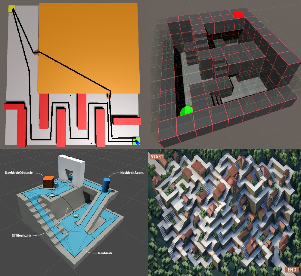
In this Part of the project we implemented a reinforcement learning algorithm that would be able to solve the pathfinding problem. In addition to supervised and unsupervised learning, reinforcement learning is one of the three pillars of machine learning. In contrast to supervised, reinforcement learning does not have any labeled training data. The training process is relatable to how humans and animals learn. It is a combination of trying out and applying knowledge gained. Basically, reinforcement learning consists of an agent who works in an environment, much like a mouse in a maze. The mouse has to find a way to the end of the maze and can find something to eat as a reward. The longer the mouse explores the maze, the more experience it gains and the faster and more error-free it finishes subsequent runs.

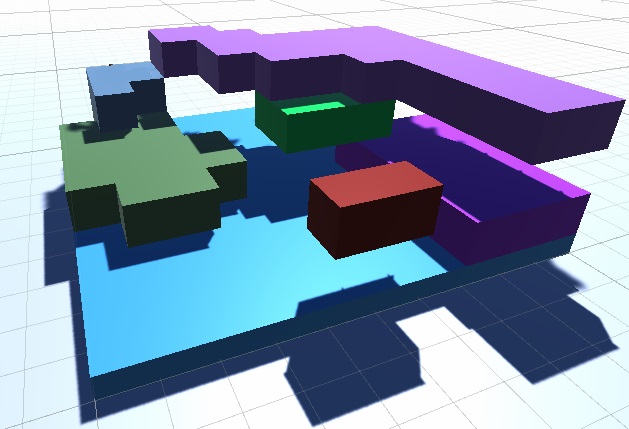
Like all reinforcement learning algorithms, ours has the essential components that are needed. Firstly the environment that contains information about the state and all the rules of how to move inside the world and how to calculate the rewards. Rewards are a numerical value, which qualify the actions taken. In the first implementation the world was also part of the environment, but we figured out that only the position of the agent is vital. The world never changes its voxels, so it does not need to be stored. Secondly the agent, who interacts with the environment and gets rewards depending on the actions taken.

While in training, the environment gets an action. Each action received is called a step and all steps, accumulated until some break up criteria are met, are called an episode. Before the action gets executed, it gets examined. If the action leads to an invalid state, then the action is denied, the episode will be ended, a final reward is calculated and the environment will reset to its original state. If the action is valid, then the action is executed, the state will be updated, and a reward is calculated and accumulated to the previous rewards of this episode.

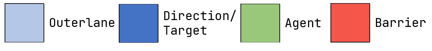
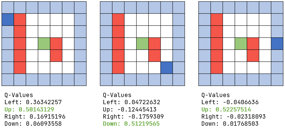
There are 4 ways in total how an episode can be ended. First of all, with an illegal move, like walking into a wall. A second option is reaching the goal. The third way is reaching the maximum number of steps allowed per episode. The last to trigger the end is reaching the minimum reward cap. Each action has a corresponding reward depending on the state of the environment. Walking into a wall gives a highly negative reward - while walking in general gives a very minor negative reward. This shall encourage the agent to find the shortest path. Another minor negative reward is given when the agent walks onto a cell which was already visited in this episode. Lastly there is a negative reward given depending on the general distance to the target. The closer the agent is to the target, the smaller is the negative reward. Moving onto the target cell is the only positive reward the agent can get. One integral part of Reinforcement Learning is the Q-Net. This Q-Net is a deep neural network which contains Q-Values which are calculated from the relation of state, action and reward. Its main purpose is to provide information for the markov decision process, which in return selects the optimal action to maximize the reward for all subsequent steps in an episode. While in training, the Q-Net gets updated with experiences from the replay buffer and an optimizer to minimize a cost function. The replay buffer is a list in which every finished episode is stored, while in training, some of the episodes inside the replaybuffer are then selected and used to update the policy of the agent. 
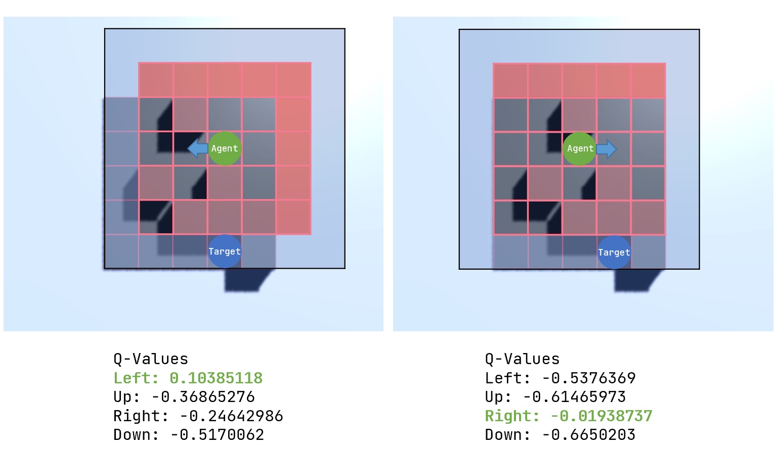
A policy is a strategy that the agent uses to accomplish its task. Based on the experiences learned, the policy dictates how the agent behaves under certain conditions. Conditions in this project would be the position of the agent. The optimizer used in this project is the ADAM optimizer, adaptive moment estimation, which is an extension of the SGD algorithm, stochastic gradient descent. The agent is the entity which is interacting with the environment. It contains the Q-Net, an optimizer and a loss function. There are two types of agents which are in use. The first is a DQN-agent, which has a deep neural network instead of plain Q-table, which is used in Q-learning and it is trained with episodes of the replay buffer. The Other is a DDQN-agent, which uses two identical deep neural networks.

While in training there are two different modi on how an action is selected. Exploring, the agent gets random actions without using its knowledge and it is mainly used in the beginning of the training. This eventually leads to new paths and prevents the agent from getting stuck. Later on the agent will rely more on the exploitation and uses the accumulated knowledge to improve the paths found so far.

Many different hyperparameters can be tuned for the training process. The epsilon value, discount factor, learning rate, size of the replaybuffer, number of episodes, number of steps per episode, number of neural network layers, number of nodes for the layers and the values for the individual rewards.
The epsilon value expresses the ratio of exploration to exploitation. A value of 0.1 means that in one out of ten episodes the agent gets random actions. The discount factor, a value between zero and one, describes whether the agent is more long term or short term oriented. The learning rate represents how much the Q-net gets updated in each iteration. A value of zero would indicate no learning at all and a value of one overrides old Q-Values with the new ones. Finding the optimal set of hyperparameters is very complex because the training involves a lot of randomness during the exploration phase. A direct before and after comparison is not always meaningful because of this.

Our setup is based on Tensorflow and it’s TF-Agents library. It provides a lot of performant modular solutions to implement reinforcement learning projects. The most positive aspect is the significant speed boost in training an agent, which is due to how Tensorflow works and how efficiently it processes its datastreams. If the correct version of it is installed, the Nvidia CUDA toolkit is automatically used to accelerate the training process using the available GPU resources.

Transfer Learning

Our reinforcement learning approach has one major problem, which restricts the possible use cases: It can only learn one world with one start and goal. Therefore we came up with a concept to create an agent that knows its way around, even in worlds it has never seen before. This transfer learning approach was only implemented in 2D space to save computation time when generating the data and training the model.

The general idea is that the agent in each state knows how to do local pathfinding within small subsections of a world based on the target’s general direction. We decided to use a 5x5 field of view (FOV). In addition, the direction of the global target for the world is stored in each FOV, so that the agent knows in which direction it has to move in order to reach the target. If the global target is within the FOV, the corresponding position is marked as the direction. The same combination of FOV and target direction can occur in multiple worlds. Ideally, an agent who can handle all those combinations, knows its way around any world, even those it has never seen.

In order to be able to implement this concept, we divided the process into four steps:

Transfer learning progress
  • In the first step, 5x5 FOVs are created from variously sized, generated worlds. Then a 5x5 FOV is generated for every possible free agent position. Positions outside of the world are marked as walls in the FOV at the edges. Different sized worlds are used to generate the FOVs in order to be able to provide as many different FOVs as possible, since our world generating algorithm increases the size of the obstacles with the size of the world. In order not to store a FOV twice in the data set, a unique hash is generated for each FOV. If the hash of a FOV is already present in the dataset, it will be discarded. Alternatively, 5x5 worlds could have been generated directly and used as FOVs. The difference is that the overall voxel distribution of a newly generated 5x5 world could differ a lot from how an actual, bigger world would look like. So generating FOVs out of the target worlds could produce better results as it will more accurately represent the pathfinding challenges inside the smaller FOV.
Field of view creation out of a world
  • In the next step, all FOVs are extended by an outer lane containing only free fields, resulting in 7x7 FOVs. This is necessary to be able to store the direction of the global target of the entire world in the FOV, since the target will not always be within. Then, for each extended FOV, for all free fields as a target, reinforcement learning is used to calculate a path. Based on that, the Q-values for the actions Left, Top, Right and Bottom at the position of the center of the FOV are predicted. We always predict only the Q-values for the center, since this is the only position we’re going to care about, that is the position of the agent.
Iteration over all possible directions

With this information, the agent can decide for each FOV’s center and each possible direction (based on the global target) which action is most likely the best to take.

Q-Values for different directions in a field of view

The resulting training data for the model are 2-tuples each with the 7x7 FOV with the marked direction for the global target and the 4 Q-values of the center of the FOV.

  • Next we train a convolutional neural network using the generated data, via supervised learning. For this we pass the FOVs of the training data as input to the model and the corresponding Q-values as labels. After the training, the model is able to output the appropriate Q-values based on incoming FOVs with a marked direction.
  • In the last step we use the trained model to predict paths in unknown worlds. For this purpose, a 5x5 FOV is created based on the agent’s position in the entire world, extended by the outer lane. The direction of the global target is marked at the correct position in the FOV.The model predicts the Q-values for the current position based on this 7x7 FOV. The agent executes the action with the highest Q-value and the process is repeated for the resulting agent position. This procedure is repeated until either the target is reached or a specified number of steps is exceeded.

Limitations

One weakness of our transfer learning approach is the possibility that the agent jumps back and forth between two fields and thus gets stuck. This happens if the agent at position X, for example, decides to move to the right, based on the Q-values and at the next position X+1 the Q-value for the action to move to the left is the highest. This problem arises from the fact that the agent cannot completely overlook a large obstacle in its 5x5 FOV and thus decides for a path to a goal, which can be invalid in the next step, because on the path that was still valid in the previous FOV, there is suddenly a wall.

Example of an agent repeatedly moving from left to right, getting stuck
Problem of the limited field of view (FOV). Both paths have the same length and are valid for the current FOV

To solve this problem there are two possible approaches:

  • The FOV could be enlarged so that an obstacle can be completely overlooked in the FOV. In this case, however, the FOV would have to grow each time the obstacles become larger.
  • A better solution is an additional logic for the agent, whereby it does not always select only the action with the highest Q-value. For example, the agent could save which fields of the world have already been visited and which action was taken there. When the agent returns to a field that has already been visited, it selects the action with the next highest Q-value that has not yet been taken. This approach would prevent the back and forth jumping behavior.

Advantages over GANs and reinforcement learning

The transfer learning approach can find paths in worlds of any size in which it can survey the obstacles in its FOV (maximum 4x4 large obstacles), independent of start and target positions. An example of such a world is the custom world illustrated in the Features: World Generator chapter. In worlds of this type, the approaches with GANs and reinforcement learning fail for sizes bigger than 25x25, while transfer learning can even handle worlds of the size 50x50 and larger.

[1] medium.com [2] Buildings and steps maze pintrest